BIOPOLE - Chukchi Sea metatranscriptomics analysis report

Author

Nathan

This report summarises the bioinformatics workflow applied to the Chukchi Sea eRNA samples to study the Nitrogen cycles, particularly the denitrifcation and anammox metabolic pathways, using metatranscriptomics approach.

🧪 Sample Processing, Sequencing & Data Availability

The Centre for Genomic Research (CGR) processed 9 marine eRNA samples (+ 1 negative control) for metatranscriptomic sequencing as part of project SSP203072. The workflow included:

  • DNase treatment of all extracted RNA samples.

  • rRNA depletion using the Seawater riboPOOL kit.

  • Construction of Illumina RNA-seq libraries from the rRNA-depleted material.

Multiplexing of all libraries and sequencing on one lane of an Illumina NovaSeq X Plus (NovaSeq X+) 25B flow cell.

This setup is expected to produce approximately ~325 million read pairs per sample, providing deep metatranscriptomic coverage suitable for resolving nitrogen-cycling pathways, including denitrification and anammox.

Funding & administrative details:

  • SSP ID: SSP203072

  • Platform: Illumina NovaSeq X+

  • Funding: NEOF1819 — Purchase Order P11212-200

All files—including raw data, processing details, and download instructions—are available via:

Project data download

📊 Sequencing Output & CGR QC Summary

Name Raw Reads (M) Trimmed Reads (M) Raw Bases (M) Trimmed Bases (M)
1-S4S 422.03 418.30 126,608.75 120,507.35
2-S4M 559.84 557.67 167,952.06 163,451.31
3-S4B 613.03 611.42 183,908.71 179,372.50
4-S13S 9.89 7.81 2,968.42 2,244.11
5-S13M 240.41 238.67 72,124.26 70,520.45
6-S13B 617.78 615.94 185,334.01 181,063.09
7-S14S 526.76 524.35 158,026.71 153,976.49
8-S14M 526.33 524.19 157,899.00 153,074.61
9-S14B 571.17 569.59 171,349.89 166,325.31
10-negative_control 5.92 5.16 1,776.58 1,487.48

Description of Methods The raw FASTQ files are trimmed for the presence of Illumina adapter sequences using Cutadapt version 4.5 . The option -O 3 was used, meaning that trimming occurred in reads where at least 3bp of adapter sequence was observed at the 3’ end of the read. The reads were further trimmed to remove low quality bases with a minimum window quality score of 20. After trimming, reads shorter than 15 bp were removed. Only read pairs are retained, therefore if a read of a pair is trimmed away then the other read in the pair is also discarded.

Note📝 Notes on Low-Yield Samples

4-S13S returned an exceptionally low number of reads because very little RNA was recovered from the corresponding Sterivex filters. This limited input material resulted in poor library complexity and low overall sequencing yield.

10-negative_control is a processing negative control sample and therefore contains no biological RNA. The very low read count is expected and confirms that minimal contamination occurred during library preparation.

🧪 Bioinformatics Workflow

rRNA Removal – SortMeRNA

To enrich for mRNA and other non-rRNA transcripts, we removed ribosomal RNA using SortMeRNA.

The command below shows the SortMeRNA run that was used for each sample. We used the CGR-trimmed paired-end reads as input and the smr_v4.3_sensitive_db_rfam_seeds database for rRNA identification.

Code
sortmerna \
  --ref "smr_v4.3_sensitive_db_rfam_seeds.fasta" \
  --reads "$R1" \
  --reads "$R2" \
  --threads "$SLURM_CPUS_PER_TASK" \
  --fastx \
  --out2 \
  --paired_in \
  --aligned "${SAMPLE}_rRNA" \
  --other "${SAMPLE}_RNA_clean" \
  --workdir "$WORKDIR"

For each sample, SortMeRNA produces:

rRNA files containing reads classified as rRNA

RNA_clean files containing the rRNA-depleted read pairs, which are carried forward to assembly.

De Novo Assembly – MEGAHIT

We performed a co-assembly of selected rRNA-depleted samples using MEGAHIT, optimised for complex metatranscriptomic data with the meta-sensitive preset. For illustration, the command below shows the co-assembly of samples:

Code
megahit 
-1 [station_samples]_RNA_clean_fwd.fq.gz 
-2 [station_samples]_RNA_clean_rev.fq.gz 
-t 60 
--presets meta-sensitive 
--min-contig-len 500 
-m 0.9 
-o St[1:3]_megahit_out

Assembly statistics for an example MEGAHIT run (St1) were obtained using seqkit:

Code
seqkit stats final.contigs.fa

For example (St1 assembly):

Assembly # Contigs Total Length (bp) Min Length (bp) Mean Length (bp) Max Length (bp)
final.contigs.fa 1,432,902 1,457,453,119 500 1,017.1 106,426

These statistics indicate a highly fragmented but deep assembly, typical of complex marine microbial metatranscriptomes, with contigs ≥500 bp retained for downstream analyses.

Read Mapping – Bowtie2 and Samtools

To quantify transcript coverage across assembled contigs, we mapped the rRNA-depleted reads back to the MEGAHIT assembly using Bowtie2, followed by BAM processing with Samtools.

First, we built a Bowtie2 index from the fixed assembly:

Code
bowtie2-build St1_assembly-fixed.fa St1_assembly-fixed

Then, for each sample, paired-end reads were aligned and processed as follows:

Code
IDX="St1_assembly-fixed"
R1="SAMPLE_RNA_clean_fwd.fq.gz"
R2="SAMPLE_RNA_clean_rev.fq.gz"
THREADS=16
OUT="St1_SAMPLE"

Map paired-end reads

bowtie2 -x "${IDX}"
-1 "${R1}"
-2 "${R2}"
-p "${THREADS}"
-S "${OUT}.sam"

Convert to BAM, keep mapped reads only (-F 4), sort and index

samtools view -F 4 -bS "${OUT}.sam" -o "${OUT}-RAW.bam"
samtools sort -@ "${THREADS}" "${OUT}-RAW.bam" -o "${OUT}.bam"
samtools index "${OUT}.bam"

The resulting sorted and indexed BAM files (.bam, .bam.bai) are used as input for downstream coverage estimation and gene- or contig-level quantification in anvi’o.

Creating anvi’o Databases

Subsequent steps involved importing the assemblies and mapped reads into anvi’o to facilitate contig profiling, annotation, and interactive exploration of nitrogen-cycle genes (e.g. denitrification and anammox pathways).

In brief, the workflow included:

  1. Creating a contigs database from the MEGAHIT assembly

  2. Running HMMs and functional annotation (e.g. PFAM, TIGRFAMs, KOfam)

  3. Profiling BAM files for each sample to obtain coverage and detection statistics

  4. Merging profiles across samples for joint inspection and downstream analyses

Example (commands will vary slightly depending on environment and anvio version):

  1. Create contigs database
Code
anvi-gen-contigs-database -f St1_assembly-fixed.fa -o St1_contigs.db -n "St1 Chukchi Sea metaT"
  1. Run HMMs (standard anvio collection)
Code
anvi-run-hmms -c St1_contigs.db --num-threads 20
  1. Profile each BAM file
Code
anvi-profile -i St1_SAMPLE.bam -c St1_contigs.db
--output-dir St1_SAMPLE_profile
--num-threads 20
  1. Merge profiles across samples
Code
anvi-merge St1_*_profile/PROFILE.db -o St1_merged_profiles -c St1_contigs.db

These anvi’o databases form the basis for functional annotation and visualisation of key nitrogen-cycle pathways in the Chukchi Sea metatranscriptomes.

🔍 Functional Annotation of genes

To characterise the metabolic potential represented in the metatranscriptomic assembly, we performed extensive functional annotation of the anvi’o contigs database. This step links assembled sequences to known protein families, orthologous groups, and taxonomic markers, enabling downstream interpretation of nitrogen-cycle genes (e.g., denitrification, anammox).

We used the following anvi’o annotation programs:

Code
anvi-run-hmms

Identifies single-copy core genes (SCGs) and key conserved protein families using anvi’o’s curated HMM collections. This provides quality metrics for assemblies and forms the basis for taxonomic inference.

Code
anvi-run-ncbi-cogs

Assigns Clusters of Orthologous Groups (COGs) from NCBI to contigs based on predicted open reading frames. COG categories help identify broad functional roles such as energy production, amino acid metabolism, stress response, etc.

Code
anvi-run-kegg-kofams

Annotates genes using KEGG Orthologs (KOfam HMMs), providing pathway-level information including nitrogen cycling modules (e.g., nitrate reduction, nitrification, denitrification, anammox).

Code
anvi-run-scg-taxonomy

Uses single-copy core gene content to infer taxonomic origin of contigs, giving insight into which microbial groups are contributing to specific nitrogen-cycling pathways.

🔬 Metabolic Reconstruction and Pathway Visualisation

Following functional annotation, we performed metabolic inference and pathway-level analysis using anvi’o’s metabolism suite. These tools integrate KEGG Ortholog (KOfam) annotations with curated pathway models to identify which biochemical pathways are represented in the dataset and to visualise how transcripts map onto specific metabolic processes—particularly those involved in nitrogen cycling.

We used the following anvi’o programs:

Code
anvi-estimate-metabolism

Identifies complete and partial KEGG modules across all annotated contigs, providing an overview of metabolic potential (e.g., denitrification, dissimilatory nitrate reduction, anammox).

Code
anvi-reaction-network

Generates reaction-centric metabolic networks based on KEGG reactions detected in the assembly. This allows exploration of how individual reactions connect into broader nitrogen pathways.

Code
anvi-draw-kegg

Renders KEGG metabolic pathway diagrams annotated with detected genes, enabling visual inspection of pathway completeness and highlighting which steps are supported by metatranscriptomic evidence.

These tools collectively provide a pathway-level view of nitrogen cycling activity in the Chukchi Sea microbial community, enabling detailed interpretation of expression patterns associated with denitrification, nitrification, and anammox processes.

KEGG Module M00529 — Denitrification (nitrate → nitrogen)

KEGG module M00529 (Denitrification, nitrate → nitrogen). Diagram from https://www.genome.jp/dbget-bin/www_bget?md:M00529

From the output of anvi-estimate-metabolism, we can look for the KEGG module for Denitrification (M00529) and look at its completeness:

KEGG Module Station stepwise_module_completeness pathwise_module_completeness
M00529 Station_1 1.00 1.00
M00529 Station_2 1.00 1.00
M00529 Station_3 1.00 1.00

So all the genes required for denitrification to occur seem to be detected at each of the stations.

Let’s look at the denitrification pathway in more details using anvi-interactive, so we can see the coverage of the genes involved in denitrification across the 3 depths in the stations.

First, we need to create an anvi’o collection that contains all the denitrification genes. Using anvi-export-functions we can get the gene_callers_ids matching your KO IDs, then we can get the contigs name using anvi-export-table –table genes_in_contigs. After that we need to use join to find the contigs that have the genes of interest and finally we need to add “_split_00001” to each contig name (because in this case each contig has only one split as these come from metaT assembly. We ad a column with the name of our bin and then can import that using anvi-import-collection

Station 1

Code
anvi-export-functions   -c St1_contigs.db   -o St1_gene_functions.tsv
anvi-export-table --table genes_in_contigs -o St1_genes_in_contigs.tsv St1_contigs.db
tail -n +2 St1_genes_in_contigs.tsv | cut -f1,2 > gene_to_contig.tsv

# KO list for denitrification (edit/add as needed)
KOS='K00370|K00371|K00374|K02567|K02568|K00368|K15864|K04561|K02305|K00376'
# Get unique gene_callers_id hits for those KOs
awk -F'\t' -v kos="$KOS" '($3 ~ kos){print $1}' St1_gene_functions.tsv   | sort -u > genes_of_interest.ids
join -t $'\t' genes_of_interest.ids gene_to_contig.tsv   | cut -f2   | sort -u > contigs_of_interest.txt
awk '{print $1"_split_00001\tdenitrification"}' contigs_of_interest.txt   > denitrification_splits_collection.tsv

anvi-import-collection   -p St1_MERGED/PROFILE.db   -c St1_contigs.db   -C denitrification_splits denitrification_splits_collection.tsv

Now that we have an anvio collection, we need to “split” it from the main contigs and profile databases (we create a subset). This is because our initial contigs.be has too many splits (1,432,906 splits to be precise) and hierarchical clustering gets turned off.

Once it is splitted we can find a directory called “denitrifications_splits” in which we find a contigs and profile database that we can now plot using anvi-interactive.

First, we will import the data about the presence/absence of the genes of interest (from Module M00529) so we can visualise where they are found.

Code
anvi-export-functions   -c CONTIGS.db   -o gene_functions.tsv
anvi-export-table --table genes_in_contigs -o genes_in_contigs.tsv CONTIGS.db

# 1) Define your KO list (space-separated)
KOS="K00370 K00371 K00374 K02567 K02568 K00368 K15864 K04561 K02305 K00376"

# 2) Build gene-level KO presence/absence from gene_functions.tsv (KO is column 3)
awk -F'\t' -v OFS='\t' -v kos="$KOS" '
BEGIN{
    n = split(kos, k, " ")
    for (i=1; i<=n; i++) KO[k[i]] = 1
    printf "gene_callers_id"
    for (i=1; i<=n; i++) printf "%s%s", OFS, k[i]
    printf "\n"
}
NR==1 { next }  # skip header
{
    gene = $1
    acc  = $3
    genes[gene] = 1
    if (acc in KO) present[gene, acc] = 1
}
END{
    for (g in genes) {
        printf "%s", g
        for (i=1; i<=n; i++) {
            ko = k[i]
            v = ((g SUBSEP ko) in present) ? 1 : 0
            printf "%s%d", OFS, v
        }
        printf "\n"
    }
}
' gene_functions.tsv > KO_presence_absence_by_gene.tsv

# 3) Map gene_callers_id -> contig (requires genes_in_contigs.tsv from anvi-export-gene-calls)
#    Then collapse to contig-level by OR (max) across genes
awk -F'\t' -v OFS='\t' '
NR==FNR {
    if (FNR==1) next
    gene2contig[$1] = $2
    next
}
FNR==1 { print "contig", substr($0, index($0, "\t")+1); ncol=NF; next }
{
    gene = $1
    contig = (gene in gene2contig) ? gene2contig[gene] : "NA"
    contigs[contig]=1
    for (i=2; i<=NF; i++) if ($i==1) M[contig, i]=1
}
END{
    for (c in contigs) {
        printf "%s", c
        for (i=2; i<=ncol; i++) {
            v = ((c SUBSEP i) in M) ? 1 : 0
            printf "%s%d", OFS, v
        }
        printf "\n"
    }
}
' genes_in_contigs.tsv KO_presence_absence_by_gene.tsv > KO_presence_absence_by_contig.tsv

# 4) Convert contig names to split names (naive: appends _split_00001)
awk -F'\t' -v OFS='\t' '
FNR==1 { $1="item_name"; print; next }
{ $1 = $1 "_split_00001"; print }
' KO_presence_absence_by_contig.tsv > KO_presence_absence_by_split.tsv

# Import the data to the PROFILE.db
anvi-import-misc-data -p PROFILE.db -t items KO_presence_absence_by_split.tsv

anvi’o interactive plot - Denitrification

Anvi’o interactive plot showing the presence/absence of transcript annotation associated with denitrification in station 1.

From this plot we see that:

  1. K00370 (narG) and K00371 (narH) are annotated on the same transcript (bin 1 on figure) which makes sense as they are subunits of the same nitrate reductase enzyme complex. In many bacterial genomes, narG and narH are directly adjacent and commonly co-transcribed as part of a nitrate reductase operon. For example, in E. coli the nar operon appears to contain four genes designated narGHJI (https://pmc.ncbi.nlm.nih.gov/articles/PMC211023/pdf/jbacter00182-0317.pdf).Operons are typically transcribed as one long mRNA. Hence, having multiple functions on one transcript here is not surprising.

  2. Transcripts are annotated with the same gene multiple times. Different microbial populations likely have slightly different sequences for these genes, hence they get assembled into multiple different versions instead of collapsed by the assembler into one sequence. Hence, having multiple transcript with the same function is not surprising.

From the coverage data layers, we can see that all the transcripts have coverage from sample S4B (Bottom) and most for sample S4M (Mid-water) but some might be missing from sample S4S (Surface). Therefore, let’s look at the completeness of denitrification per depth instead of for the whole station.

Code
anvi-estimate-metabolism -c CONTIGS.db -p PROFILE.db -O denitrification_meta --add-coverage

From the output table we see that, the denitrification module (M00529) shows differences in both abundance (average coverage) and completeness (average detection) across samples. St1_S4S exhibits substantially lower coverage and detection, indicating a reduced presence and/or partial representation of the denitrification pathway in the surface sample. In contrast, St1_S4M and St1_S4B show much higher coverage and detection values, consistent with a more abundant and more complete denitrification potential in deeper waters. Notably, St1_S4B shows the highest detection, suggesting the most complete representation of the pathway among the three samples. Given that denitrification is surely happening in the sediments, this result makes sense.

Sample Avg. Coverage Avg. Detection
St1_S4S 975.53 0.454
St1_S4M 2032.39 0.787
St1_S4B 1706.59 0.859

The table below provides a gene-level breakdown of the denitrification module (KEGG M00529), linking each predicted gene (Gene_ID) to its corresponding KEGG Ortholog (KO) and its sequencing coverage in three samples (St1_S4B, St1_S4M, and St1_S4S).

Gene_ID KO St1_S4B_coverage St1_S4M_coverage St1_S4S_coverage
1359363 K00368 20.27 20.03 0.00
691166 K00368 165.50 334.52 13.32
707695 K00368 41.86 69.14 12.56
687620 K00368 1282.92 2415.36 243.79
700737 K00368 2478.69 2384.15 1253.82
854256 K00368 11.42 3.33 5.35
1185346 K00368 28.96 5.83 7.43
941749 K00368 38.13 27.69 5.36
1709903 K00368 105.23 88.92 34.86
1705673 K00368 344.46 682.02 178.39
65438 K00368 6.36 5.16 6.08
1031617 K00368 689.90 1204.79 165.63
26013 K00368 12.50 12.82 15.19
1787639 K00368 9.67 18.67 17.90
888296 K00368 40.10 45.63 5.36
895831 K00368 49445.22 52866.89 44637.37
882932 K00368 14.22 18.09 8.26
87959 K00368 10915.16 11415.02 4717.44
994614 K00368 1.93 17.48 0.00
1617538 K00368 14.71 12.26 18.99
1348289 K00368 19.23 17.71 3.41
411974 K00368 12.60 27.54 0.00
441287 K00368 145.19 279.39 10.43
516928 K00368 14.62 4.14 0.00
19512 K00368 9.06 9.22 0.00
189833 K00368 16223.04 32930.34 3152.75
443514 K00368 34.88 66.09 4.25
823538 K00368 935.07 1874.67 392.60
1814075 K00368 69.73 164.82 0.00
742645 K00370 878.67 1009.92 251.12
594150 K00371 2.45 14.29 6.35
1363937 K00371 10.21 3.34 16.68
815415 K00371 0.75 9.27 26.97
85995 K00371 7687.83 7547.90 2080.32
144516 K00371 55.76 69.10 41.32
433983 K00371 8190.78 7206.54 2536.75
528599 K00371 1780.68 1350.22 893.72
742644 K00371 691.15 522.57 229.56
772410 K00371 12746.27 12521.72 4925.97
894284 K00371 523.03 645.82 215.08
1228756 K00371 78.42 116.44 19.89
747852 K00374 17.94 5.84 32.57
123437 K00374 4.63 7.16 29.05
815414 K00374 0.00 8.06 24.44
474316 K00374 1.32 6.27 3.20
123436 K00374 0.00 4.48 18.10
1743784 K00376 11.08 4.67 1.33
296938 K00376 23.40 8.46 4.35
239047 K00376 16.09 8.26 3.63
110498 K00376 5.29 8.14 0.00
374090 K00376 9.87 1.92 0.00
793456 K00376 8.94 0.00 0.00
921128 K00376 9.35 4.09 0.00
1401364 K02305 8.46 3.23 0.00
1445710 K02305 14.92 16.69 2.89
1753152 K02567 11.96 9.67 4.48
1433084 K02567 12.63 2.15 0.00
1852908 K02567 4.25 2.22 20.11
1168575 K02568 5.91 11.02 1.58
648640 K02568 5.24 2.09 0.00
1431702 K02568 7.02 4.45 0.00
481953 K02568 18.70 19.84 0.00
685198 K04561 17.10 0.22 0.00
1271679 K04561 11.50 3.54 0.00
468297 K04561 11.63 5.93 0.00
252981 K04561 21.79 1.74 29.56
540786 K04561 3.42 7.74 0.72
1468402 K15864 9.09 5.81 5.57

Multiple gene copies are associated with several key denitrification steps, indicating some degree of functional redundancy within the pathway. Gene coverages are generally higher in St1_S4B and St1_S4M than in St1_S4S, where several components show low or zero coverage, suggesting a reduced or incomplete representation of the pathway in this sample. A small number of genes display particularly high coverage, implying that certain denitrification functions may be more prevalent than others across the dataset.

Now using the table above, we can list for each sample the Gene_IDs and KOs with nonzero coverage and we can turn that list into into an enzymes-txt file which can be used to calculated the denitrification completeness score for each sample, using:

Code
anvi-estimate-metabolism --enzymes-txt
Sample Module Step Path Unique_prop Unique_enzymes Hits
St1_S4S M00529 1 1 1 K00376, K02305, K04561 3, 1, 2
St1_S4M M00529 1 1 1 K00376, K02305, K04561 6, 2, 5
St1_S4B M00529 1 1 1 K00376, K02305, K04561 7, 2, 5

All three samples (St1_S4S, St1_S4M, and St1_S4B) show complete denitrification pathways according to both stepwise and pathwise KEGG module criteria, indicating that all required enzymatic steps from nitrate to N₂ are represented.

The number of hits for the unique enzymes differs among samples. St1_S4B and St1_S4M show higher hit counts for most of the unique enzymes compared to St1_S4S, suggesting that these functions are represented by more gene transcripts or more abundant RNAs in these samples.

Together, these results suggest that the denitrification pathways is fully expressed in all three samples, but its relative transcription representation appears to be lower in St1_S4S than in St1_S4M and St1_S4B.

Station 2

anvi’o interactive plot - Denitrification

Anvi’o interactive plot showing the presence/absence of transcript annotation associated with denitrification in station 2.
Code
anvi-estimate-metabolism -c CONTIGS.db -p PROFILE.db -O denitrification_meta --add-coverage

Station 2 - denitrification module (M00529) - Overall Coverage and Detection

Sample Avg. Coverage Avg. Detection
St2_S13M 591.48 0.267
St2_S13B 744.24 0.987
gene_id KO St2_S13B_coverage St2_S13M_coverage
931374 K00368 10.08 0.00
918819 K00368 15.68 0.00
1418801 K00368 163.54 43.36
1738715 K00368 43.83 0.00
2523618 K00368 41.43 11.64
2113065 K00368 22.97 12.42
786120 K00368 216.51 0.00
2206329 K00368 54.89 92.86
1618381 K00368 26.37 5.56
1590745 K00368 99.84 45.48
1584359 K00368 42.60 44.68
2424048 K00368 114.98 44.27
414561 K00368 4494.64 5765.92
435135 K00368 70.35 21.38
2362307 K00368 710.15 542.33
541901 K00368 3614.32 2636.43
531120 K00368 36.83 11.95
562266 K00368 2.19 0.00
322701 K00368 251.78 377.37
630301 K00368 974.45 969.33
574423 K00368 92.67 196.61
2171711 K00368 14.44 0.00
877233 K00368 89.64 180.05
1185798 K00368 28.05 32.23
1624701 K00368 93.27 0.00
666396 K00368 623.03 720.09
837789 K00368 43830.05 38809.44
2290077 K00368 9119.11 8907.05
1696038 K00368 54.14 5.20
2458663 K00368 17.06 0.00
719725 K00368 26.35 0.00
174546 K00368 50.02 10.36
168770 K00368 3125.79 3178.60
463269 K00368 26.42 27.78
506383 K00368 4.91 0.00
798212 K00368 10.50 0.00
985890 K00368 47.27 0.00
1270286 K00368 5727.33 7407.03
1480719 K00368 27.67 0.00
1521983 K00368 57.02 73.18
1561147 K00368 18.99 0.00
1639940 K00368 14.65 0.00
1850275 K00368 7.92 0.63
1866615 K00368 163.49 7.60
2172851 K00368 81.96 83.78
2519190 K00368 114.06 3.05
210469 K00370 350.70 96.54
659566 K00370 99.00 46.66
912139 K00370 15.96 14.37
2065205 K00370 61.61 0.00
344188 K00371 8.10 0.00
343404 K00371 85.34 11.39
419316 K00371 1270.89 401.22
594548 K00371 44.55 0.02
659565 K00371 30.89 79.39
677555 K00371 89.77 50.80
686644 K00371 52.34 0.11
774869 K00371 317.11 24.94
937882 K00371 2431.67 801.01
1014350 K00371 121.05 0.00
1094781 K00371 15727.85 8005.47
1306759 K00371 384.99 90.60
1824372 K00371 384.44 52.99
2065206 K00371 56.63 0.00
2085985 K00371 7659.48 4453.23
2096924 K00371 389.66 261.85
2241189 K00371 2560.98 730.70
2332334 K00371 99.99 14.77
1956955 K00376 12.60 0.00
1708452 K00376 16.28 0.00
161373 K00376 18.09 0.00
791462 K00376 21.08 0.00
1787011 K00376 24.13 0.00
1987182 K00376 14.47 0.00
2391504 K00376 41.63 0.00
598544 K00376 16.27 0.00
393052 K00376 13.38 0.00
40339 K00376 14.60 0.00
163373 K00376 16.59 38.95
189553 K00376 11.02 0.00
310667 K00376 10.48 0.00
534673 K00376 6.51 0.00
583293 K00376 11.19 0.00
631195 K00376 8.44 0.00
841939 K00376 10.83 0.00
1081191 K00376 11.32 0.00
1204882 K00376 8.83 0.00
1425850 K00376 8.34 0.00
1764210 K00376 9.08 0.00
1825774 K00376 17.02 0.00
1874322 K00376 7.85 0.00
2430721 K00376 23.36 19.52
524270 K02305 27.63 0.00
744452 K02305 7.52 0.59
2106842 K02305 10.50 0.00
288202 K02305 18.20 25.04
574195 K02305 21.96 5.31
371414 K02305 18.94 0.24
865141 K02305 9.94 0.00
854645 K02305 29.91 0.00
2343082 K02305 16.41 5.70
813369 K02305 23.38 0.00
1590238 K02305 5.02 20.89
1961121 K02567 16.40 23.37
1080629 K02567 26.07 0.00
2013728 K02567 9.63 0.00
915792 K02568 17.28 0.00
1421858 K02568 10.71 0.00
1435882 K02568 14.32 0.00
2530302 K02568 16.28 20.26
965607 K02568 12.49 0.00
2015867 K02568 4.11 0.00
1991999 K02568 21.12 0.00
2061765 K02568 11.34 0.00
2412112 K02568 14.45 0.00
1878822 K02568 9.54 39.78
599773 K02568 1.72 0.00
659599 K02568 25.65 0.00
678080 K02568 3.64 0.00
1240323 K04561 10.27 16.97
1022160 K04561 16.66 2.18
496996 K04561 12.03 17.42
742859 K04561 18.95 4.07
773984 K04561 9.30 0.00
2572937 K04561 22.64 0.00
1821176 K04561 17.37 0.00
2210362 K04561 38.83 12.73
2018951 K04561 21.55 0.00
1601181 K04561 11.98 0.00
2425700 K04561 23.40 0.00
2422413 K04561 18.74 0.00
2388297 K04561 12.56 79.95
120712 K04561 28.89 10.33
98994 K04561 13.86 0.00
546096 K04561 13.94 0.00
391276 K04561 14.61 0.00
22156 K04561 4.82 17.17
838930 K04561 11.23 0.00
1688715 K04561 14.25 0.00
997108 K04561 5.05 0.00
1883166 K04561 12.88 0.00
1966268 K04561 29.11 0.00
1603792 K15864 29.66 0.00
1631676 K15864 10.64 0.00
2005999 K15864 18.37 0.00
Sample Module Step Path Unique_prop Unique_enzymes Hits
St2_S13M M00529 1 1 1 K00376, K02305, K04561 2, 6, 8
St2_S13B M00529 1 1 1 K00376, K02305, K04561 24, 11, 23

Station 3

anvi’o interactive plot - Denitrification

Anvi’o interactive plot showing the presence/absence of transcript annotation associated with denitrification in station 3.

Station 3 - denitrification module (M00529) - Overall Coverage and Detection

Sample Avg. Coverage Avg. Detection
St3_S14S 575.89 0.363
St3_S14M 3178.61 0.626
St3_S14B 1897.44 0.910
Gene_ID KO St3_S14B_coverage St3_S14M_coverage St3_S14S_coverage
940220 K00368 3038.25 12004.95 2326.99
1141487 K00368 1751.71 1089.09 45.87
696726 K00368 15.40 71.61 8.40
1524063 K00368 4680.11 17604.95 2732.90
103044 K00368 1.39 28.20 13.24
1603484 K00368 6728.30 6164.95 875.79
1688623 K00368 11994.78 5892.07 252.05
1397102 K00368 24.10 13.22 3.30
430064 K00368 1288.07 603.14 35.30
161749 K00368 34.05 32.39 14.07
158371 K00368 10843.19 20992.16 5862.66
1833581 K00368 496.66 307.37 58.01
603080 K00368 12285.39 24752.47 2451.92
749765 K00368 23810.01 36314.16 13077.81
830637 K00368 17101.34 29621.69 4860.73
888098 K00368 4977.08 13838.97 1409.40
1017872 K00368 2542.48 967.99 40.87
1265105 K00368 739.87 1711.33 230.75
1656914 K00368 9.18 14.02 30.43
1514788 K00370 1.19 11.05 21.75
1517667 K00371 6.98 4.38 17.39
1063936 K00371 17.74 4.46 20.10
384530 K00371 318.73 84.80 5.81
413339 K00371 919.49 1081.89 74.07
727004 K00371 1970.41 3632.48 90.00
856298 K00371 57.31 90.48 18.17
1386808 K00371 4.23 10.38 42.01
1807011 K00371 9006.75 16658.33 488.65
1137166 K00374 7.05 11.42 3.91
1749377 K00374 15.87 28.42 14.24
1386807 K00374 0.75 9.90 2.84
Sample Module Step Path Unique_prop Unique_enzymes Hits
St3_S14S M00529 0.5 0.5 NA No enzymes unique to module NA
St3_S14M M00529 0.75 0.875 1 K00376, K04561 1, 2
St3_S14B M00529 1 1 1 K00376, K02305, K04561 3, 2, 8
NoteDepth-related patterns in denitrification potential at Station 3

The completeness of the KEGG denitrification module (M00529; nitrate → N₂) increased with depth at Station 3, indicating a clear vertical gradient in the transcript presence/abundance for this pathway. In the surface sample (St3_S14S), the module showed low completeness (stepwise = 0.5, pathwise = 0.5), suggesting that only partial denitrification steps, such as nitrate or nitrite reduction, may be present in the community. The absence of enzymes unique to the module further indicates that the full denitrification pathway is likely incomplete at this depth.

In contrast, the mid-water sample (St3_S14M) exhibited higher completeness (stepwise = 0.75, pathwise = 0.875), with detection of enzymes specific to the later stages of denitrification, including nitric oxide reductase (K04561) and nitrous oxide reductase (K00376). This suggests that organisms capable of performing most steps of denitrification are present in the mid-water microbial community.

The bottom sample (St3_S14B) showed full pathway completeness (stepwise = 1, pathwise = 1), with multiple hits for enzymes involved in the terminal steps of denitrification. The detection of key enzymes such as nitrous oxide reductase (K00376) and nitric oxide reductase (K02305, K04561) indicates that the microbial community likely possesses the capacity to carry out complete denitrification, potentially converting nitrate to dinitrogen gas.

Overall, these results suggest a depth-dependent increase in denitrification potential, with incomplete or partial pathways in surface waters and a fully represented pathway in deeper layers. This pattern suggests that denitrification is influenced by the proximity with the sediments and/or with the amount of particles which relates to the fact that denitrification becomes more favorable under low-oxygen or anoxic conditions.

Summary

denitrification pathway steps:

NO₃⁻ → NO₂⁻ → NO → N₂O → N₂

Typical KO groups:

Step Enzyme Gene KO
Nitrate → Nitrite Nitrate reductase narG / napA K00370, K02567
Nitrite → NO Nitrite reductase nirK / nirS K00368, K15864
NO → N₂O Nitric oxide reductase norB K04561
N₂O → N₂ Nitrous oxide reductase nosZ K00376
Accessory nos genes nosD/F/Y K02305
Sample Avg Coverage Avg Detection Stepwise Completeness Pathwise Completeness Unique Prop. Unique Enzymes (hit)
St1_S4S 975.53 0.454 1.00 1.00 1 K00376 (3), K02305 (1), K04561 (2)
St1_S4M 2032.39 0.787 1.00 1.00 1 K00376 (6), K02305 (2), K04561 (5)
St1_S4B 1706.59 0.859 1.00 1.00 1 K00376 (7), K02305 (2), K04561 (5)
St2_S13M 591.48 0.267 1.00 1.00 1 K00376 (2), K02305 (6), K04561 (8)
St2_S13B 744.24 0.987 1.00 1.00 1 K00376 (24), K02305 (11), K04561 (23)
St3_S14S 575.89 0.363 0.50 0.50 NA No enzymes unique to module
St3_S14M 3178.61 0.626 0.75 0.875 1 K00376 (1), K04561 (2)
St3_S14B 1897.44 0.910 1.00 1.00 1 K00376 (3), K02305 (2), K04561 (8)

Heatmap of denitrification gene coverage across stations and depths.

Values correspond to log-transformed gene coverage

Denitrification pathway diagram (KEGG ortholog map
NoteDiscussion

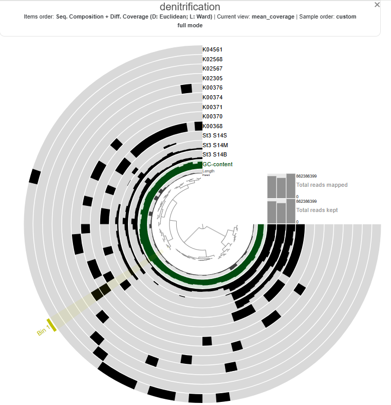
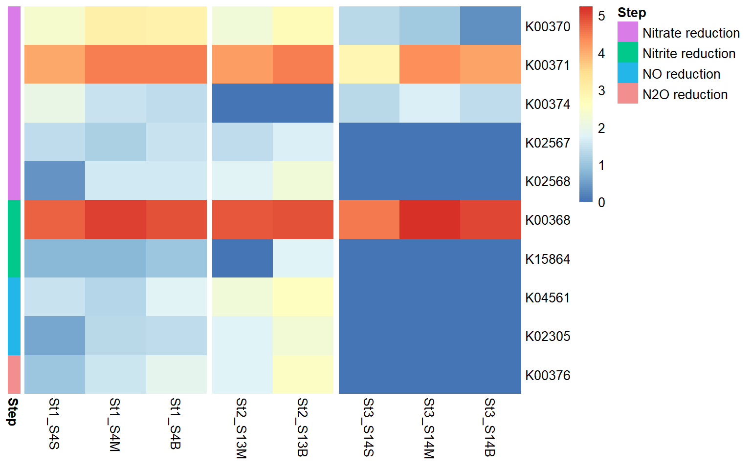
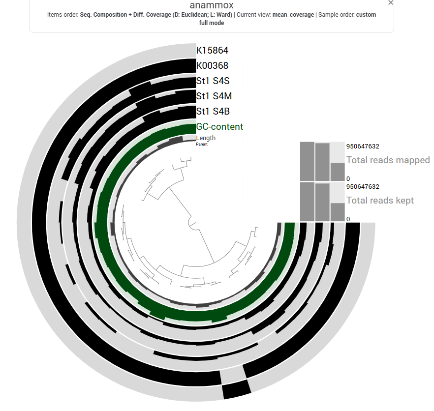
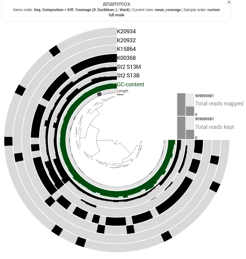
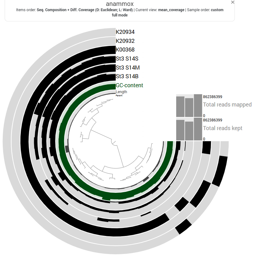
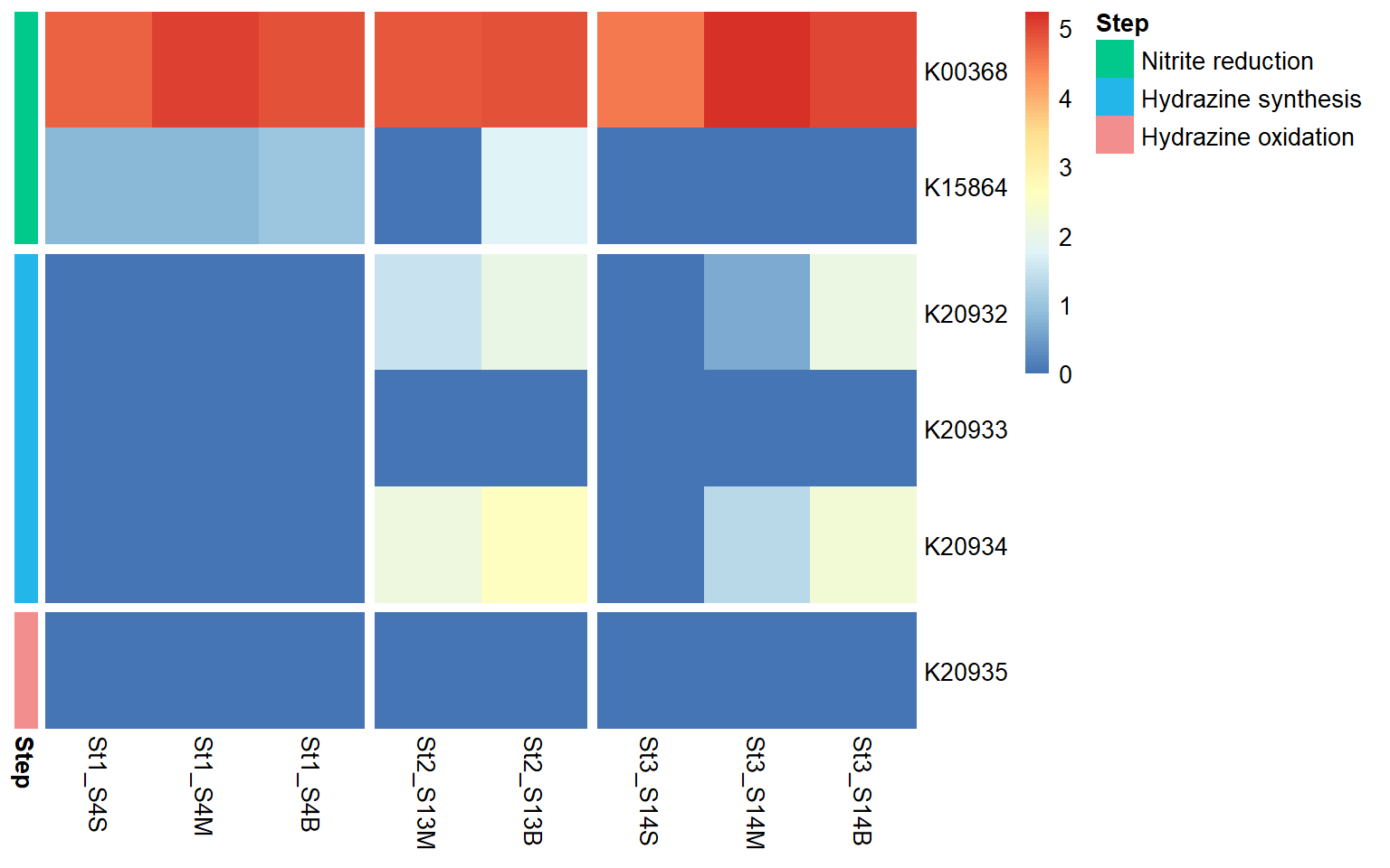
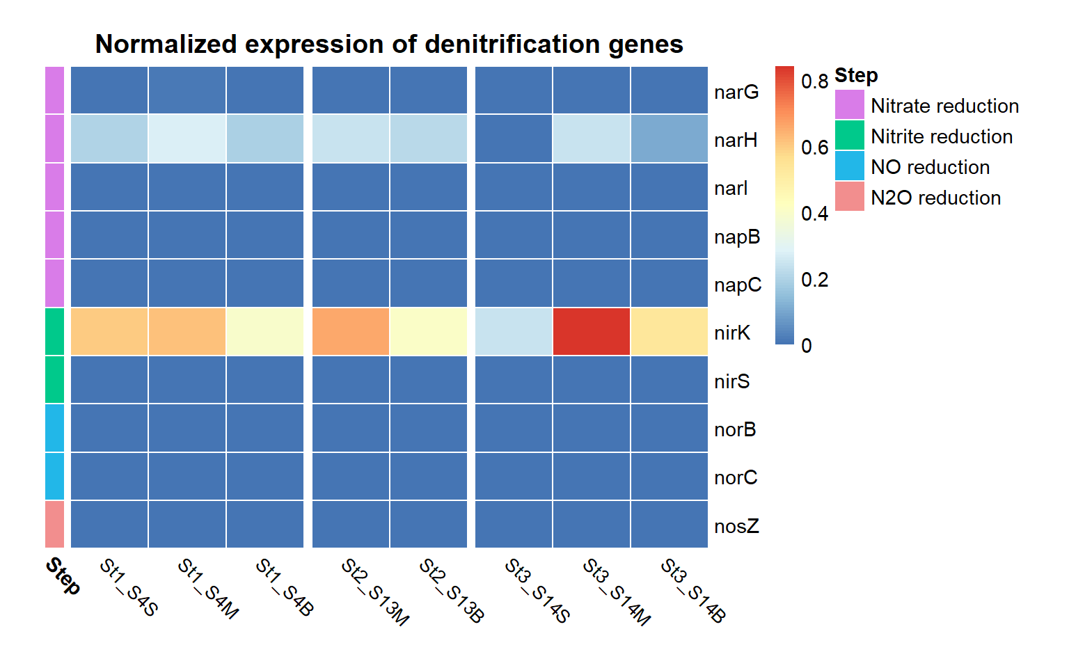
The heatmap shows the distribution and relative expression of denitrification-related KEGG orthologs (KO) genes across the stations and depth layers. Overall, the results indicate substantial spatial variability in the transcription of denitrification genes across the study area.

Nitrate reduction genes

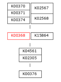
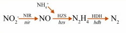
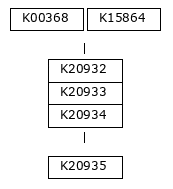
The first step of denitrification, the reduction of nitrate to nitrite, can be catalyzed by two distinct enzymatic systems: the membrane-bound nitrate reductase (Nar) and the periplasmic nitrate reductase (Nap). In this dataset, the Nar pathway is represented by K00370, K00371, and K00374, while the Nap pathway is represented by K02567 and K02568 (see pathway diagram above).

At Station 1, transcripts from both nitrate reduction systems (Nar and Nap) are detected.At Station 2, K00374 is absent, indicating only partial expression of the Nar-associated genes detected in this dataset, while with both the Nap genes K02567 and K02568, the Nap pathwa is complete. In contrast, Station 3 shows limited expression of Nar genes and Nap-associated transcripts are absent, indicating reduced transcription of nitrate-to-nitrite reduction pathways at this station.

Nitrite reduction genes

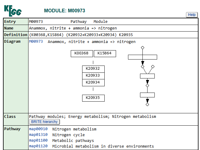
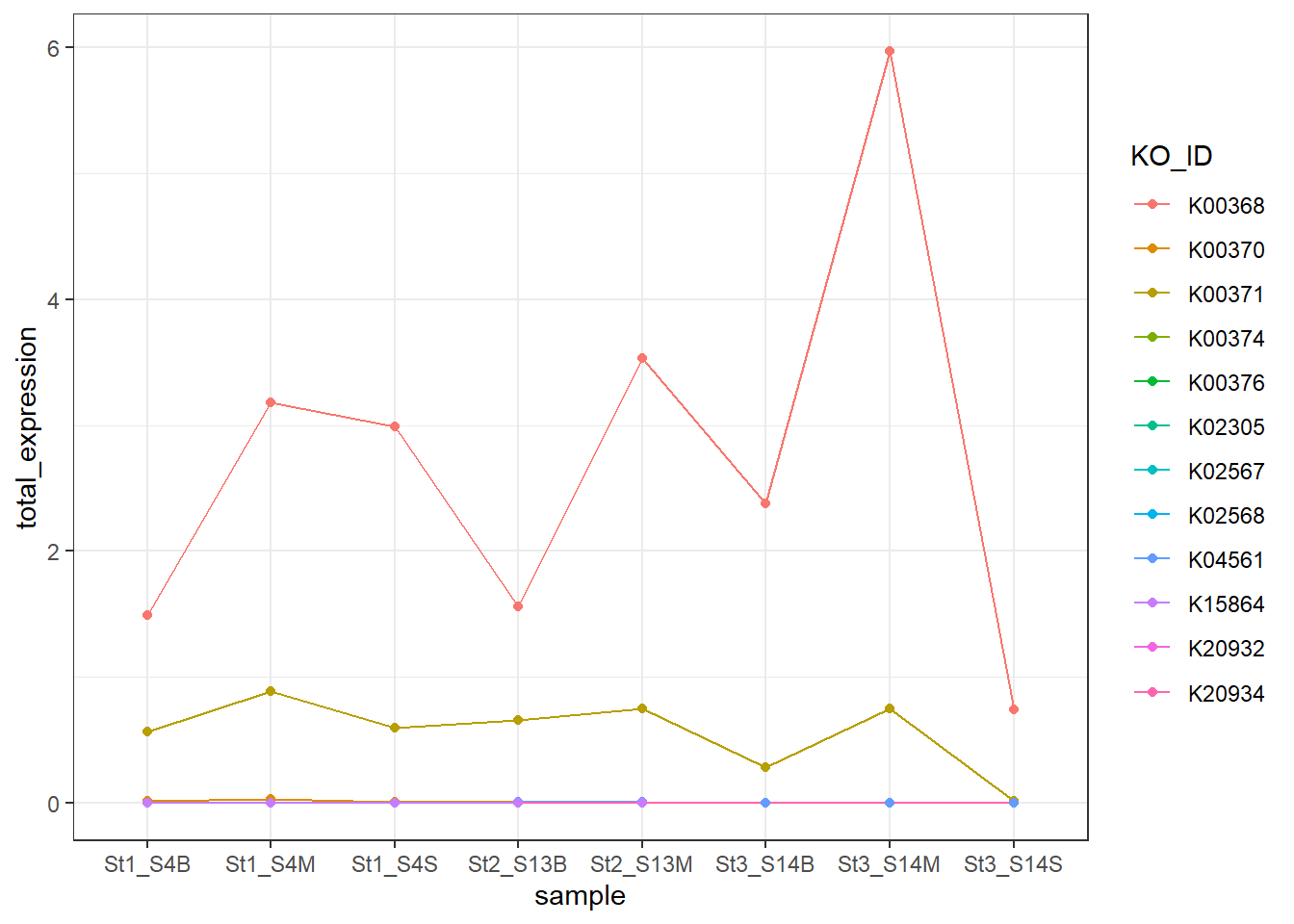
Genes associated with the reduction of nitrite to nitric oxide are represented by K00368 (nirK) and K15864 (nirS), which encode alternative nitrite reductases (the presence of only one transcript is enough). The gene of nirK exhibits the highest coverage across samples, indicating that the conversion of nitrite to nitric oxide may represent a dominant step in the denitrification pathway in these samples. In contrast, nirS shows considerably lower expression, suggesting a predominance of nirK-type denitrifiers in the active microbial assemblages.

Nitric oxide reduction genes

Genes involved in the reduction of nitric oxide to nitrous oxide are represented by K04561 (norB) and K02305 (norC), which are associated with the nitric oxide reductase system. The heatmap shows moderate transcript coverage at Stations 1 and 2, with the highest expression observed in the mid-water and bottom samples at Station 2. This suggests that the nitric oxide reduction step of denitrification is actively transcribed at Stations 1 and 2, particularly in deeper waters, whereas expression of nitric oxide reductase genes appears to be minimal at Station 3.

Nitrous oxide reduction gene

The final step of denitrification, the reduction of nitrous oxide to dinitrogen gas, is represented by K00376 (nosZ), alone. Transcripts of this gene are detected primarily at Stations 1 and 2, indicating that microorganisms capable of reducing nitrous oxide may be transcriptionally active in these environments. However, expression levels remain relatively moderate compared with earlier steps of the pathway, and transcripts are largely absent at Station 3, suggesting limited expression of this step at that station.

Depth-related patterns

Across Stations 1 and 2, several denitrification genes exhibit higher transcript levels in mid-water and bottom samples compared to surface waters, suggesting that denitrification activity may be enhanced in deeper parts of the water column.

Anammox (anaerobic ammonium oxidation) - KEGG Module M00973

Overall process: nitrite + ammonia → nitrogen gas

KEGG module M00973 — Anammox (anaerobic ammonium oxidation). Diagram from https://www.genome.jp/dbget-bin/www_bget?md:M00973
Step Requirement Function
1 K00368 OR K15864 Nitrite reduction
2 K20932 + K20933 + K20934 Hydrazine synthase complex
3 K20935 Hydrazine dehydrogenase

Anammox reaction

Let’s do the same workflow as for denitrification.

From the output of anvi-estimate-metabolism, we can look for the KEGG module for Anammox (M00973) and look at its completeness for each of the stations:

KEGG Module Station stepwise_module_completeness pathwise_module_completeness
M00973 Station_1 0.33 0.33
M00973 Station_2 0.33 0.55
M00973 Station_3 0.33 0.55

The KEGG module for anaerobic ammonium oxidation (anammox; M00973) was incomplete at all three sampling stations. While transcripts associated with nitrite reduction (K00368 and/or K15864) were detected across the datasets, the key hydrazine synthase complex and hydrazine dehydrogenase required for a functional anammox pathway were not fully present. Stepwise module completeness was therefore low (0.33) for all stations, indicating no transcript evidence for a complete anammox pathway in these samples (Table 1).

Table 1. Presence of key genes/transcripts associated with the anammox pathway (KEGG module M00973) across the three stations.

Gene (KO) Function Station 1 Station 2 Station 3
K00368 / K15864 Nitrite reduction
K20932 Hydrazine synthase subunit A
K20933 Hydrazine synthase subunit B
K20934 Hydrazine synthase subunit C
K20935 Hydrazine dehydrogenase

The absence of both the complete hydrazine synthase complex (subunit A, B and C) and the hydrazine dehydrogenase suggests that the canonical anammox pathway is not supported by the metatranscriptomics data at any of the sampled stations.

Still, let’s look at the distribution of these genes/transcripts across the differents depths of our 3 stations.

NoteNote

The nitrite reductase genes (K00368 or K15864) detected in the samples are shared between anammox and denitrification pathways.

Station 1

Code
# KO list for anammox-specific genes
KOS='K00368|K15864|K20932|K20933|K20934|K20935'

# Get unique gene_callers_id hits for those KOs
awk -F'\t' -v kos="$KOS" '($3 ~ kos){print $1}' St1_gene_functions.tsv \
  | sort -u > genes_of_interest.ids
  
sort -k1,1 gene_to_contig.tsv > gene_to_contig.sorted.tsv

join -t $'\t' genes_of_interest.ids gene_to_contig.sorted.tsv \
  | cut -f2 \
  | sort -u > contigs_of_interest.txt

awk '{print $1"_split_00001\tanammox"}' contigs_of_interest.txt \
  > anammox_splits_collection.tsv

anvi-import-collection \
  -p St1_MERGED/PROFILE.db \
  -c St1_contigs.db \
  -C anammox_splits \
  anammox_splits_collection.tsv
Code
anvi-export-functions   -c CONTIGS.db   -o gene_functions.tsv
anvi-export-table --table genes_in_contigs -o genes_in_contigs.tsv CONTIGS.db

# 1) Define your KO list (space-separated)
KOS="K00368 K15864 K20932 K20933 K20934 K20935"

# 2) Build gene-level KO presence/absence from gene_functions.tsv (KO is column 3)
awk -F'\t' -v OFS='\t' -v kos="$KOS" '
BEGIN{
    n = split(kos, k, " ")
    for (i=1; i<=n; i++) KO[k[i]] = 1
    printf "gene_callers_id"
    for (i=1; i<=n; i++) printf "%s%s", OFS, k[i]
    printf "\n"
}
NR==1 { next }  # skip header
{
    gene = $1
    acc  = $3
    genes[gene] = 1
    if (acc in KO) present[gene, acc] = 1
}
END{
    for (g in genes) {
        printf "%s", g
        for (i=1; i<=n; i++) {
            ko = k[i]
            v = ((g SUBSEP ko) in present) ? 1 : 0
            printf "%s%d", OFS, v
        }
        printf "\n"
    }
}
' gene_functions.tsv > KO_presence_absence_by_gene.tsv

# 3) Map gene_callers_id -> contig (requires genes_in_contigs.tsv from anvi-export-gene-calls)
#    Then collapse to contig-level by OR (max) across genes
awk -F'\t' -v OFS='\t' '
NR==FNR {
    if (FNR==1) next
    gene2contig[$1] = $2
    next
}
FNR==1 { print "contig", substr($0, index($0, "\t")+1); ncol=NF; next }
{
    gene = $1
    contig = (gene in gene2contig) ? gene2contig[gene] : "NA"
    contigs[contig]=1
    for (i=2; i<=NF; i++) if ($i==1) M[contig, i]=1
}
END{
    for (c in contigs) {
        printf "%s", c
        for (i=2; i<=ncol; i++) {
            v = ((c SUBSEP i) in M) ? 1 : 0
            printf "%s%d", OFS, v
        }
        printf "\n"
    }
}
' genes_in_contigs.tsv KO_presence_absence_by_gene.tsv > KO_presence_absence_by_contig.tsv

# 4) Convert contig names to split names (naive: appends _split_00001)
awk -F'\t' -v OFS='\t' '
FNR==1 { $1="item_name"; print; next }
{ $1 = $1 "_split_00001"; print }
' KO_presence_absence_by_contig.tsv > KO_presence_absence_by_split.tsv

# Import the data to the PROFILE.db
anvi-import-misc-data -p PROFILE.db -t items KO_presence_absence_by_split.tsv

anvi’o interactive plot - Anammox

Anvi’o interactive plot showing the presence/absence of transcript annotation associated with Anammox in station 1.
Code
anvi-estimate-metabolism -c CONTIGS.db -p PROFILE.db -O anammox_meta --add-coverage
Sample Avg. Coverage Avg. Detection
St1_S4S 1830.53 0.480
St1_S4M 3567.58 0.875
St1_S4B 2771.32 0.926

The table below provides a gene-level breakdown of the anammox module, linking each predicted gene (Gene_ID) to its corresponding KEGG Ortholog (KO) and its sequencing coverage in three samples (St1_S4B, St1_S4M, and St1_S4S).

Gene_ID KO St1_S4B_coverage St1_S4M_coverage St1_S4S_coverage
1359363 K00368 20.27 20.03 0.00
691166 K00368 165.50 334.52 13.32
707695 K00368 41.86 69.14 12.56
687620 K00368 1282.92 2415.36 243.79
700737 K00368 2478.69 2384.15 1253.82
854256 K00368 11.42 3.33 5.35
1185346 K00368 28.96 5.83 7.43
941749 K00368 38.13 27.69 5.36
1709903 K00368 105.23 88.92 34.86
1705673 K00368 344.46 682.02 178.39
65438 K00368 6.36 5.16 6.08
1031617 K00368 689.90 1204.79 165.63
26013 K00368 12.50 12.82 15.19
1787639 K00368 9.67 18.67 17.90
888296 K00368 40.10 45.63 5.36
895831 K00368 49445.22 52866.89 44637.37
882932 K00368 14.22 18.09 8.26
87959 K00368 10915.16 11415.02 4717.44
994614 K00368 1.93 17.48 0.00
1617538 K00368 14.71 12.26 18.99
1348289 K00368 19.23 17.71 3.41
411974 K00368 12.60 27.54 0.00
441287 K00368 145.19 279.39 10.43
516928 K00368 14.62 4.14 0.00
19512 K00368 9.06 9.22 0.00
189833 K00368 16223.04 32930.34 3152.75
443514 K00368 34.88 66.09 4.25
823538 K00368 935.07 1874.67 392.60
1814075 K00368 69.73 164.82 0.00
1468402 K15864 9.09 5.81 5.57

Now using the table above, we can list for each sample the Gene_IDs and KOs with nonzero coverage and we can turn that list into into an enzymes-txt file which can be used to calculated the anammox completeness score for each sample, using:

Code
anvi-estimate-metabolism --enzymes-txt
Sample Module Step Path Unique_prop Unique_enzymes Hits
St1_S4S M00973 0.33 0.33 NA No enzymes unique to module NA
St1_S4M M00973 0.33 0.33 NA No enzymes unique to module NA
St1_S4B M00973 0.33 0.33 NA No enzymes unique to module NA

IMPORTANT NOTE: with no enzymes unique to module, the values of coverage and detection above are actually missleading as they inform us about enzymes that are also involved in order pathways than anammox. Probably it would be better to use only enzymes that are unique to modules for both denitrification and anammox! here we would have zero for coverage and detection of anammox given that none of the enzymes exclusively used in the pathway are present!

Station 2

anvi’o interactive plot - Anammox

Anvi’o interactive plot showing the presence/absence of transcript annotation associated with Anammox in station 2.
Sample Avg. Coverage Avg. Detection
St2_S13M 1214.26 0.99
St2_S13B 1293.10 0.40

The table below provides a gene-level breakdown of the anammox module, linking each predicted gene (Gene_ID) to its corresponding KEGG Ortholog (KO) and its sequencing coverage in the two samples of station 2 (St2_S13B and St2_S13M).

Gene_ID KO St2_S13B_coverage St2_S13M_coverage
931374 K00368 10.08 0.00
918819 K00368 15.68 0.00
1418801 K00368 163.54 43.36
1738715 K00368 43.83 0.00
2523618 K00368 41.43 11.64
2113065 K00368 22.97 12.42
786120 K00368 216.51 0.00
2206329 K00368 54.89 92.86
1618381 K00368 26.37 5.56
1590745 K00368 99.84 45.48
1584359 K00368 42.60 44.68
2424048 K00368 114.98 44.27
414561 K00368 4494.64 5765.92
435135 K00368 70.35 21.38
2362307 K00368 710.15 542.33
541901 K00368 3614.32 2636.43
531120 K00368 36.83 11.95
562266 K00368 2.19 0.00
322701 K00368 251.78 377.37
630301 K00368 974.45 969.33
574423 K00368 92.67 196.61
2171711 K00368 14.44 0.00
877233 K00368 89.64 180.05
1185798 K00368 28.05 32.23
1624701 K00368 93.27 0.00
666396 K00368 623.03 720.09
837789 K00368 43830.05 38809.44
2290077 K00368 9119.11 8907.05
1696038 K00368 54.14 5.20
2458663 K00368 17.06 0.00
719725 K00368 26.35 0.00
174546 K00368 50.02 10.36
168770 K00368 3125.79 3178.60
463269 K00368 26.42 27.78
506383 K00368 4.91 0.00
798212 K00368 10.50 0.00
985890 K00368 47.27 0.00
1270286 K00368 5727.33 7407.03
1480719 K00368 27.67 0.00
1521983 K00368 57.02 73.18
1561147 K00368 18.99 0.00
1639940 K00368 14.65 0.00
1850275 K00368 7.92 0.63
1866615 K00368 163.49 7.60
2172851 K00368 81.96 83.78
2519190 K00368 114.06 3.05
1603792 K15864 29.66 0.00
1631676 K15864 10.64 0.00
2005999 K15864 18.37 0.00
211939 K20932 70.11 9.41
1757114 K20932 29.94 21.46
967270 K20934 45.53 22.50
57397 K20934 110.83 19.01
143245 K20934 30.75 0.00
487771 K20934 79.50 17.80
555311 K20934 19.95 15.02
1044587 K20934 21.91 0.00
1221553 K20934 59.47 54.13

Now using the table above, we can list for each sample the Gene_IDs and KOs with nonzero coverage and we can turn that list into into an enzymes-txt file which can be used to calculated the anammox completeness score for each sample.

Sample Module Step Path Unique_prop Unique_enzymes Hits
St2_S13M M00973 0.33 0.55 1 K20932, K20934 2, 5
St2_S13B M00973 0.33 0.55 1 K20932, K20934 2, 7

Station 3

anvi’o interactive plot - Anammox

Anvi’o interactive plot showing the presence/absence of transcript annotation associated with Anammox in station 3.
Sample Avg. Coverage Avg. Detection
St3_S14S 1214.26 0.99
St3_S14M 1214.26 0.99
St3_S14B 1293.10 0.40

The table below provides a gene-level breakdown of the anammox module, linking each predicted gene (Gene_ID) to its corresponding KEGG Ortholog (KO) and its sequencing coverage in the two samples of station 2 (St2_S13B and St2_S13M).

Gene_ID KO St3_S14B_coverage St3_S14M_coverage St3_S14S_coverage
940220 K00368 3038.25 12004.95 2326.99
1141487 K00368 1751.71 1089.09 45.87
696726 K00368 15.40 71.61 8.40
1791053 K00368 34.76 10.59 0.00
1524063 K00368 4680.11 17604.95 2732.90
103044 K00368 1.39 28.20 13.24
1603484 K00368 6728.30 6164.95 875.79
1738209 K00368 7.60 14.89 0.00
1545927 K00368 35.29 33.19 0.00
1688623 K00368 11994.78 5892.07 252.05
1397102 K00368 24.10 13.22 3.30
254326 K00368 220.22 1.24 0.00
259217 K00368 4.79 27.96 0.00
600787 K00368 103.68 33.79 0.00
591293 K00368 15.86 7.15 0.00
430064 K00368 1288.07 603.14 35.30
161749 K00368 34.05 32.39 14.07
158371 K00368 10843.19 20992.16 5862.66
1833581 K00368 496.66 307.37 58.01
492060 K00368 6.77 6.70 0.00
603080 K00368 12285.39 24752.47 2451.92
749765 K00368 23810.01 36314.16 13077.81
830637 K00368 17101.34 29621.69 4860.73
888098 K00368 4977.08 13838.97 1409.40
1012201 K00368 8.58 19.55 0.00
1017872 K00368 2542.48 967.99 40.87
1265105 K00368 739.87 1711.33 230.75
1375753 K00368 15.44 6.23 0.00
1656914 K00368 9.18 14.02 30.43
1249493 K20932 58.06 1.49 0.00
1703483 K20932 57.86 2.19 0.00
845486 K20934 82.04 17.55 0.00
155944 K20934 69.44 2.12 0.00
624237 K20934 39.44 0.00 0.00

Now using the table above, we can list for each sample the Gene_IDs and KOs with nonzero coverage and we can turn that list into into an enzymes-txt file which can be used to calculated the anammox completeness score for each sample.

Sample Module Step Path Unique_prop Unique_enzymes Hits
St3_S14S M00973 0.33 0.33 NA No enzymes unique to module NA
St3_S14M M00973 0.33 0.55 1 K20932, K20934 2, 2
St3_S14B M00973 0.33 0.55 1 K20932, K20934 2, 3

Summary

Anammox pathway steps:

NO₂⁻ → NO → N₂H₄ → N₂

In addition, NH₄⁺ is consumed in the key step:

NO + NH₄⁺ → N₂H₄

Typical KO groups:

Step Enzyme Gene KO
Nitrite → Nitric oxide Nitrite reductase nirK / nirS K00368, K15864
NO + NH₄⁺ → Hydrazine Hydrazine synthase hzsA / hzsB / hzsC K20932, K20933, K20934
Hydrazine → N₂ Hydrazine dehydrogenase hdh K20935
Sample Avg Coverage Avg Detection Stepwise Completeness Pathwise Completeness Unique Prop. Unique Enzymes (hit)
St1_S4S 975.53 0.454 1.00 1.00 1 K00376 (3), K02305 (1), K04561 (2)
St1_S4M 2032.39 0.787 1.00 1.00 1 K00376 (6), K02305 (2), K04561 (5)
St1_S4B 1706.59 0.859 1.00 1.00 1 K00376 (7), K02305 (2), K04561 (5)
St2_S13M 591.48 0.267 1.00 1.00 1 K00376 (2), K02305 (6), K04561 (8)
St2_S13B 744.24 0.987 1.00 1.00 1 K00376 (24), K02305 (11), K04561 (23)
St3_S14S 575.89 0.363 0.50 0.50 NA No enzymes unique to module
St3_S14M 3178.61 0.626 0.75 0.875 1 K00376 (1), K04561 (2)
St3_S14B 1897.44 0.910 1.00 1.00 1 K00376 (3), K02305 (2), K04561 (8)

Heatmap of anammox gene coverage across stations and depths.

Values correspond to log-transformed gene coverage

Anammox pathway diagram (KEGG ortholog map
NoteDiscussion

The heatmap shows the distribution and relative expression of anammox-related KEGG orthologs (KO) genes across the stations and depth layers.

Transcripts corresponding to the nitrite reduction genes K00368 and K15864 were detected in several samples, with K00368 showing relatively high expression across all stations. However, these genes are not specific to anammox metabolism and are also involved in other nitrogen cycling processes such as denitrification. Therefore, their expression alone does not indicate active anammox activity.

Transcripts corresponding to two subunits of the hydrazine synthase complex (K20932 and K20934) were detected in samples from Stations 2 and 3, particularly in deeper samples. Hydrazine synthase is a key enzyme unique to anammox metabolism, suggesting that transcripts related to this process are present in these communities. However, the K20933 subunit was not detected, and transcripts for hydrazine dehydrogenase (K20935), which catalyses the final step of the anammox pathway, were absent across all samples.

Because both the complete hydrazine synthase complex and hydrazine dehydrogenase are required for a functional anammox pathway, the metatranscriptomic data do not provide evidence for the full expression of the canonical anammox pathway in these samples. The detected transcripts may reflect partial expression of related enzymes, low-abundance anammox taxa, or homologous genes involved in other nitrogen transformation processes.

Overall, the results suggest that while some anammox-associated transcripts are present—particularly in deeper samples at Stations 2 and 3—the absence of key pathway components indicates that active anammox metabolism is unlikely to be fully expressed in these communities at the time of sampling.

Normalising gene coverages

Gene coverages were normalised using the housekeeping genes rpoB and gyrB, which encode the β subunit of RNA polymerase and DNA gyrase, respectively. These genes are typically present as single-copy, core components of bacterial genomes and are constitutively expressed, making them suitable proxies for baseline cellular transcriptional activity. Using the geometric mean of rpoB and gyrB provides a stable reference that accounts for variation in sequencing depth and community composition, while reducing bias associated with reliance on a single gene. This approach enables more robust comparison of denitrification and anammox gene expression across samples and depths within the water column.

Code
HK_KOS='K03043|K02470'

awk -F'\t' -v kos="$HK_KOS" '($3 ~ kos){print $1}' St1_gene_functions.tsv \
  | sort -u > housekeeping_genes.ids
  
join -t $'\t' housekeeping_genes.ids gene_to_contig.sorted.tsv \
  | cut -f2 \
  | sort -u > housekeeping_contigs.txt
  
anvi-export-gene-coverage-and-detection \
  -p St1_MERGED/PROFILE.db \
  -c St1_contigs.db \
  --genes-of-interest housekeeping_genes.ids \
  -O St1_housekeeping
  
# Let's do the same with the denitrification genes

anvi-export-gene-coverage-and-detection   -p St1_MERGED/PROFILE.db   -c St1_contigs.db   --genes-of-interest genes_of_interest.ids   -O St1_denitrification

Same for the housekeeping genes:

# A tibble: 0 × 5
# ℹ 5 variables: station <chr>, sample <chr>, rpoB_cov <dbl>, gyrB_cov <dbl>,
#   hk_geom <dbl>

Heatmap of normalized denitrification gene expression across stations and depths.

NoteDiscussion

Context and normalization approach

To assess the relative expression of denitrification genes across samples, gene coverages derived from metatranscriptomic data were normalized against housekeeping genes. Specifically, coverage values for each gene were divided by the geometric mean of the coverage of rpoB (K03043) and gyrB (K02470), two conserved single-copy genes involved in core cellular processes. This approach accounts for differences in sequencing depth and overall transcriptional activity, allowing gene expression to be interpreted relative to baseline cellular function. Normalized coverages were then summed per KEGG Orthology (KO) identifier within each sample to estimate the total community-level expression of each enzymatic step in the denitrification pathway. The resulting values were log-transformed to facilitate comparison across genes and samples with different expression magnitudes.

Interpretation of denitrification gene expression patterns The heatmap reveals that denitrification activity is dominated by the nitrite reduction step, with nirK (K00368) showing consistently higher normalized expression than other genes, particularly in mid-depth samples such as St3_S14M. In contrast, genes involved in nitrate reduction (nar and nap complexes) exhibit moderate and more uniform expression across samples, suggesting that upstream substrate availability may not be limiting. Notably, expression of nosZ (K00376), responsible for the final reduction of N₂O to N₂, is consistently low or absent, indicating that denitrification may be incomplete and potentially leading to the accumulation of nitrous oxide. Overall, the observed patterns suggest that denitrification is actively expressed in the studied water column, with pronounced variability across depths and stations, and a potential imbalance between upstream and downstream steps of the pathway.

Mapping transcripts to genomes of potential denitrifiers

The reference genomes listed in this table represent marine prokaryotes that are ecologically plausible contributors to denitrification in Arctic shelf waters such as the Chukchi Sea.

Species Phylum Class Ecological niche (marine) Denitrification relevance
Colwellia psychrerythraea Pseudomonadota Gammaproteobacteria Arctic / cold-adapted, particle-associated narGHI, nirS, norB; often incomplete (N₂O-prone)
Shewanella baltica Pseudomonadota Gammaproteobacteria Cold coastal waters, redox-flexible nar/nap, partial denitrification common
Psychromonas arctica Pseudomonadota Gammaproteobacteria Psychrophilic, organic-matter associated Nitrate reduction, variable downstream steps
Marinobacter alkaliphilus Pseudomonadota Gammaproteobacteria Marine copiotroph, particle-associated nar/nap present in many strains
Planktomarina temperata Pseudomonadota Alphaproteobacteria Free-living, bloom-associated napAB, nirS/K, norB; variable nosZ
Sulfitobacter pontiacus Pseudomonadota Alphaproteobacteria Bloom-associated Rhodobacteraceae napAB, nirS/K, norB; occasional nosZ

Mapping our RNA transcripts to the reference genomes of these marine prokarotes was not significant suggesting that these species were not abundant and/or active and/or detected.

Extraction of the community profile

According to this paper: https://doi.org/10.1080/19490976.2024.2323235, the best way to extract taxonomy from metaT reads is using the Kraken2/Bracken approach.

Code
kraken2 \
  --db /dssgfs01/scratch/ote_db/kraken/kraken_standard-16 \ 
  --threads 60 \ 
  --gzip-compressed \ 
  --report St1_S4S_report.txt \ 
  --output St1_S4S_kraken.out \ 
  --paired 1-S4S/1-S4S_RNA_clean_fwd.fq.gz 1-S4S/1-S4S_RNA_clean_rev.fq.gz
  
Code
bracken \
  -d /dssgfs01/scratch/ote_db/kraken/kraken_standard-16 \
  -i St1_S4S_report.txt \
  -o St1_S4S.bracken.F \
  -r 150 \
  -l F
Code
# 1) Convert Kraken2 output to Krona input
cut -f2,3 St1_S4S_kraken.out > St1_S4S.krona.tsv

# 2) Make the Krona HTML
ktImportTaxonomy -t 2 -m 3 -o St1_S4S_krona.html St1_S4S.krona.tsv

Approximately 17% of metatranscriptomic reads could be taxonomically classified using Kraken2 with the standard database (16 GB). Krona plots were therefore generated using classified reads only, and complementary family-level profiles were produced using Bracken.

Station 4

Station 13

Station 14

Tara Oceans Arctic data as reference

Rationale and overview

As no site-matched metagenomic data were available for these samples, a reference-based approach was adopted using publicly available metagenomic data from the Tara Oceans Arctic expedition (Station 194), representing the closest comparable marine Arctic microbial communities currently available.

Map of Station 194 of the Tara Oceans Polar Circle expedition in 2013 2:45 AM on September 8, 2013 (UTC)

Station 194 - Tara Oceans Polar Circle expedition

Field Value
BioSamples ID SAMEA4397903
ENA Run ID ERR3589571
Date/Time 2013-09-12T03:59:00Z
Latitude 73.3275
Longitude -168.8142
Depth 35
Layer DCM
Size fraction 0.22–3
Region Arctic Ocean

link to the NCBI SRA (Sequence Read Archive) Run Browser metadata page for a specific run accession (ERR3589571): https://trace.ncbi.nlm.nih.gov/Traces/index.html?view=run_browser&acc=ERR3589571&display=metadata

The EBI MGnify overview for analysis MGYA00607610 showing summary metadata and processed metagenomic results for a public datase is here: https://www.ebi.ac.uk/metagenomics/analyses/MGYA00607610#overview The assembly metadata is there: https://www.ebi.ac.uk/metagenomics/assemblies/ERZ7463204

This strategy enables the detection and quantification of expressed genes that are conserved between Arctic marine microbial communities, while acknowledging that locally specific taxa or gene variants not present in the reference dataset may not be captured.

Assembly of Tara Oceans Arctic metagenomes

Raw metagenomic reads from the Tara Oceans Arctic expedition were assembled de novo using MEGAHIT, which is optimized for large and complex metagenomic datasets. The resulting assembly produced a set of contigs representing microbial genomic fragments present in Arctic marine surface waters.

These contigs were subsequently used as a reference database for read mapping. While the Tara Oceans sampling locations do not overlap geographically with the Chukchi Sea, they provide a comprehensive representation of Arctic marine microbial diversity and metabolic potential, particularly for conserved biogeochemical pathways such as nitrogen cycling.

Metatranscriptomic read processing and mapping

Quality-filtered metatranscriptomic reads were mapped to the Tara Oceans Arctic contigs using Bowtie2 with default end-to-end alignment settings. Mapping was performed in paired-end mode to improve alignment specificity. Both concordant and discordant alignments were reported, although downstream analyses focused on concordantly mapped read pairs.

Mapping performance and alignment statistics

Across samples, overall alignment rates ranged from 15.8% to 27.3% of paired-end reads mapping to the Tara Oceans Arctic contigs. The majority of reads aligned concordantly exactly once (11–18%), with a smaller proportion aligning to multiple locations (3–6%). Discordant alignments accounted for approximately 0.5–1% of read pairs.

These mapping rates are consistent with expectations for metatranscriptomic datasets mapped to non-site-matched metagenomic references, particularly in polar marine systems where microbial communities exhibit strong spatial structure and strain-level diversity. The observed alignment patterns suggest that a substantial fraction of expressed genes in the Chukchi Sea microbial community are shared with, or closely related to, those represented in the Tara Oceans Arctic metagenomes.

Interpretation and limitations

This reference-based approach enables the identification and relative quantification of expressed genes that are conserved across Arctic marine microbial communities, including key genes involved in nitrogen cycling. However, transcripts derived from locally unique taxa or divergent gene variants absent from the Tara Oceans reference assembly are unlikely to be captured, resulting in an underestimation of total transcript diversity and expression.

Consequently, analyses based on this approach focus on relative expression patterns of nitrogen-cycle gene families represented in the reference dataset, rather than absolute transcript abundances or the absence of specific metabolic pathways. Despite these limitations, the approach provides a robust framework for exploring nitrogen cycling activity in the Chukchi Sea in the absence of site-specific metagenomic data.

Downloading MAGs from Station 194

Using the BioSamples ID (SAMEA4397903) in OMDB repository https://omdb.microbiomics.io/repository/ocean/genome-cols we can download all the MAGs that have been generated from the data of station 194.

Code
# 1) Download the catalog of all genomes and files:
curl -O https://sunagawalab.ethz.ch/share/microbiomics/ocean/db/2.0/data/catalogs/OMDBv2.0_data.tsv.gz

# 2) Unzip it
gunzip OMDBv2.0_data.tsv.gz

# 3) Use it to download the MAGs associated with SAMEA4397903
grep "TARA_SAMEA4397903_MAG_" OMDBv2.0_data.tsv | cut -f4 | xargs -n 1 curl -O

Now I want to change the name of the MAGs so they show the name of the species they have been associated to:

Code
awk -F'\t' 'NR>1 {print $1 "\t" $8}' taxonomy_mags | while IFS=$'\t' read -r id species; do
    species_clean=$(echo "$species" | tr ' /' '__')
    old="${id}.fa.gz"
    base="${species_clean}.fa.gz"

    [ -e "$old" ] || continue

    new="$base"
    n=2
    while [ -e "$new" ]; do
        new="${species_clean}_${n}.fa.gz"
        n=$((n+1))
    done

    mv "$old" "$new"
done

After unziping them all, we can generate an

Code
for i in `ls *fa | awk 'BEGIN{FS=".fa"}{print $1}'`
do
    anvi-gen-contigs-database -f $i.fa -o $i.db -T 60
    anvi-run-hmms -c $i.db -T 60
    anvi-run-ncbi-cogs -c $i.db -T 30
    anvi-run-kegg-kofams -c $i.db -T 30
    anvi-run-scg-taxonomy -c $i.db -T 30
done

Next, we need to make a TAB-delimited ‘external genomes’ file to describe these genomes and associate them with a name.

Code
echo -e "name\tcontigs_db_path" > external_genomes.txt
for db in *.db; do
    name="${db%.db}"
    echo -e "${name}\t${db}" >> external_genomes.txt
done
Code
anvi-gen-genomes-storage -e external_genomes.txt \
                         -o Tara_194_mags.db
Code
anvi-pan-genome -g Tara_194_mags-GENOMES.db --project-name Tara_194 -T 30
Code
anvi-script-add-default-collection -p Tara_194/Tara_194-PAN.db
anvi-summarize -g Tara_194_mags-GENOMES.db -p Tara_194/Tara_194-PAN.db -C DEFAULT

head -n 1 Tara_194_gene_clusters_summary.txt > denitrification_hits.txt
grep -E "K00370|K00371|K00374|K02567|K02568|K00368|K15864|K04561|K02305|K00376" Tara_194_gene_clusters_summary.txt >> denitrification_hits.txt

cut -f1-5,26 denitrification_hits.txt
unique_id gene_cluster_id bin_name genome_name gene_callers_id KOfam_ACC
123355 GC_00039248 EVERYTHING Unknown_HTCC2207_2 530 K00374
144179 GC_00060072 EVERYTHING Hel1_33_131_sp949499105 207 K00368
147231 GC_00063124 EVERYTHING SP4260_sp905182415 712 K02305

Maybe the denitrifiers were not binned into complete enough MAGs so they didn’t end in OMDB repository… Let’s check if we can find the genes in the Tara Ocean metaG dataset.

KO ID Description
K00374 Nitrate reductase gamma subunit (NarI)
K00368 Nitrite reductase (NO-forming)
K02305 Nitric oxide reductase subunit C
K04561 Nitric oxide reductase subunit B
K00376 Nitrous-oxide reductase

Note: The denitrification pathway is nearly complete. The two missing genes, K00370 (narG) and K00371 (narH), encode the catalytic subunits of the membrane-bound nitrate reductase (Nar) complex. Their absence is notable given the presence of K00374 (narI), the gamma subunit of the same enzyme complex. This suggests that the complete Nar enzyme is likely present in the environment, but that the missing subunits were not captured in the sequencing data or reconstructed during assembly, rather than being truly absent from the system.

KEGG Map of Nitrogen Pathways

KEGG map of Nitrogen metabolic pathways. Diagram from anvi’o and KEGG. In green are the genes present in anvio contig database for Station 1

KEGG nitrogen cycle (map00910)

This is a standard, widely used KO set covering:

  • Nitrification
  • Denitrification
  • DNRA
  • Anammox
  • Nitrogen fixation

Assimilatory pathways

Core nitrogen-cycle KOs (map00910)

  • Nitrogen fixation K02588 nifH K02591 nifD K02586 nifK

  • Nitrification K10944 amoA K10945 amoB K10946 amoC K10535 hao

  • Assimilatory nitrate reduction K00367 nasA K00360 nirA

  • Dissimilatory nitrate reduction (DNRA) K00362 napA K00363 napB K00370 narG K00371 narH K00374 narI K02567 nrfA K02568 nrfH

  • Denitrification K00368 nirK K15864 nirS K04561 norB K02305 norC K00376 nosZ

  • Anammox K20932 hzsA K20933 hzsB K20934 hzsC K20935 hdh